Contents
Introduction
Having learned how to perform static malware analysis using Ghidra, we now turn our attention to dynamic malware analysis, which involves executing suspicious programs in a secure and controlled environment to gather information about their runtime behaviour. As we have seen, Ghidra offers very advanced features to help us reverse engineer binary code. However, one of its known weaknesses up until release 10.0.0 (June 2021) had always been the lack of a built-in debugger. In order to observe the behaviour of suspicious malware as it executes, we are going to learn how to use a new tool this lab: the GNU Debugger (GDB).
Please note that, for this module, we are going to use the standard standalone version of GDB. It is worth pointing out, however, that both GDB and WinDbg have recently been integrated into Ghidra, so you may wish to experiment with them outside of this lab. Whichever way you choose to work in the future, the functionality is the same, as are the commands and shortcuts you learn in this lab.
Creating a Safe Execution Environment
Since dynamic malware analysis involves executing potentially malicious programs that could potentially harm your host system and/or network, it should only be carried out in a safe environment. For this module, we take care of this for you by providing learning challenges based on non-malicious binaries and giving you safe VMs to investigate real malware samples.
Looking ahead into your future career as a malware analyst, however, it is important that you familiarise yourself with different ways in which you can create a secure environment for dynamic malware analysis. This is covered in this lab’s recommended reading, and you should aim to have at least theoretical knowledge of the options available.
Basic Dynamic Analysis
Typically, after performing initial static analysis of a suspicious executable, you would proceed to basic dynamic analysis, where you execute the program in a controlled environment while monitoring how it interacts with the host system and network to understand its runtime behaviour. The table below describes the different levels at which monitoring can be configured.
| Monitoring Level | Description |
|---|---|
| Processes | Monitor the processes running in the host machine to see if any new processes are created as a result of executing the program. |
| File System | Observe how the malware interacts with the file system - are any new files created or existing files deleted/modified? |
| Registry | On Windows systems, check if new registry entries are created or existing ones modified. |
| Network | Monitor network traffic for activity generated by the program. Check if the program is listening on any open ports. |
Advanced Dynamic Analysis
Although very informative, basic dynamic analysis involves executing the program as a black box while monitoring it externally. A more powerful approach would allow you to control every step of the program’s execution while monitoring its internal state in real-time. This can be achieved by using a debugger.
You may have come across high-level graphical debuggers such as the ones which come as standard in most browsers or IDEs. They allow you to set breakpoints, step through the execution of a program line by line, and even modify dynamic values on the fly. Low-level debuggers such as GDB are pretty similar and, once you become familiar with them, you will see that the functionality available is pretty much the same. Two main differences to note are:
- instead of stepping through the source code line by line, you will step through the assembly code, instruction by instruction;
- while a lot of debuggers give you a graphical user interface, GDB is terminal-based, so it will look a little different from what you are used to.
Before we run GDB for the first time, we will change some configuration settings so our programs are disassembled using the Intel notation (GDB defaults to AT\&T).
==action: Run:==
vi ~/.gdbinit
==action: Add the following line:==
set disassembly-flavor intel
==action: Save and close the file.==
Now we are ready to start working through our first example.
==action: Create a file called simple-if-else.c and enter the following code:==
int main (void) {
   int i = 5;
   int j = 0;
   if (i > 3) {
       j = i;
   } else {
       return 1;
   }
   return 0;
}
This is the same program we used in a previous lab.
==action: Compile your code using gcc:==
gcc -m32 simple-if-else.c -o simple-if-else
==action: Now run it in gdb:==
gdb ./simple-if-else
You should see the gdb prompt as in the image below:
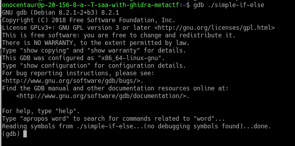 Running a program in GDB
Let’s use GDB to disassemble the program’s main function.
==action: Run:==
disassemble main
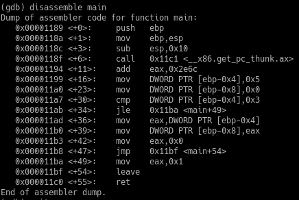 Main function disassembled in GDB
Breakpoints
You can use the break command to set a breakpoint. You can pass it a function name, a memory address, or even an offset from the function start.
==action: Let’s set a breakpoint at the start of main().== You will typically start your dynamic analysis by breaking at the start of main() in order to watch the program’s execution from the start.
==action: Type:==
break main
==action: Now run the program:==
run
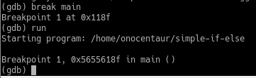 Setting a breakpoint at the start of main()
The program executed and stopped at the breakpoint. However, the default layout does not show you a lot of information.
==action: Change to the assembly layout:==
layout asm
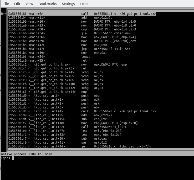 GDB showing ASM layout
Note how your view is now split: the top pane shows the disassembled code, with breakpoints indicated on the left, while the bottom pane shows the GDB console.
==action: Change to the registers layout:==
layout regs
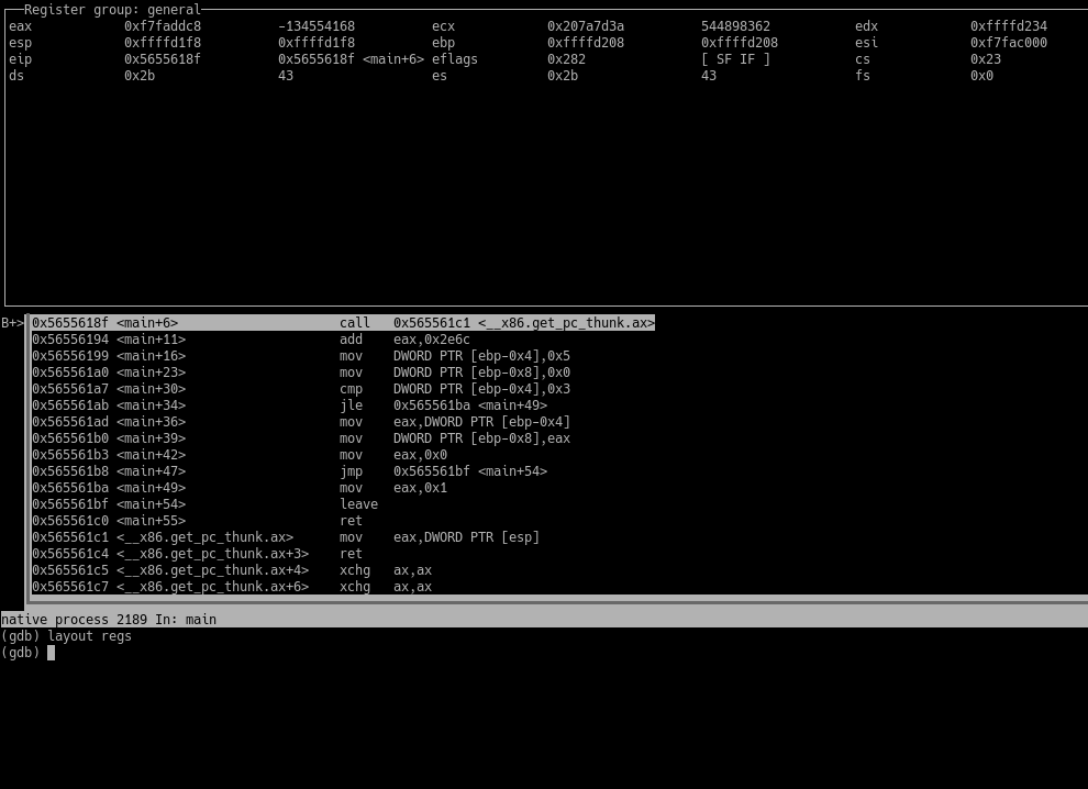 GDB showing REGS layout
This gives you an additional pane on top where you can monitor the general-purpose registers.
If we look at the disassembled code, we can see that there is a cmp instruction on line <main + 30>, followed by a jle on <main + 34>. Let’s set a breakpoint before the jle to check the results of the cmp instruction.
==action: Type:==
break *main+34
Remember: when we set a breakpoint in GDB, the program’s execution stops BEFORE the line is executed.
==action: To get a list of all the breakpoints you set, type:==
info break
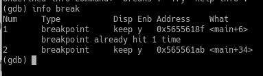 GDB showing list of breakpoints
Now that we have our second breakpoint in place, ==action: let’s continue the program’s execution.==
==action: Type:==
continue
Tip: As a shortcut, you can simply type c. For other shortcuts and a cheat-sheet of the most commonly used commands, check the reference card: GDB Quick Reference. Alternatively (and we do recommend you do this), you can create your own.
When the execution stops at our second breakpoint, we can examine the EFLAGS register to determine whether the jump will be taken or not based on the result of the preceding cmp operation. Remember the jumps table we studied in Week 4? You can use that as a reference.
According to the table, a jle jump will be taken if ZF=1 or SF=1. ==action: You can either type:==
info registers eflags
or look at the EFLAGS register information on the top pane if you are using the REGS layout.
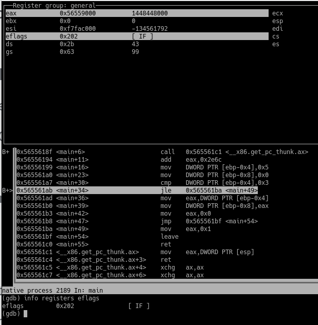 GDB showing EFLAGS register
As we can see, only the Interrupt Enabled (IF) flag is set. This is to be expected, since we are debugging. We can deduce that the jump was not taken. Let’s check if we were correct.
==action: Advance the execution by stepping exactly one instruction.==
==action: Type:==
si
Confirm that the jump was indeed not taken
Tip: You will get plenty of practice with breakpoints in this week’s CTF exercises. Don’t forget to take notes and keep a table/list of helpful commands at hand, at least until you’ve memorised them.
Examining Memory Locations
Another very useful feature of GDB (and one which you will be using a lot) is being able to examine memory locations to read the data stored in them.
==action: If you are still running the previous program in GDB, stop it by typing:==
quit
==action: Create a file called simple-types.c and enter the following code:==
#include <stdio.h>

int main(void) {
   char c = 'a';
   int i = 5;
   float f = 1.5f;
   char *name = "Rampage";
   printf("%s\n", name);
   return 0;
}
==action: Compile your code using gcc:==
gcc -m32 simple-types.c -o simple-types
==action: Now run it in gdb:==
gdb ./simple-types
==action: Add a breakpoint to the start of main().==
==action: Change the layout to ASM.==
==action: Run the program.==
Note a call to the puts() function. This is your printf() call in the original C code.
==action: Add a breakpoint on that line and continue the execution so the program stops there.==
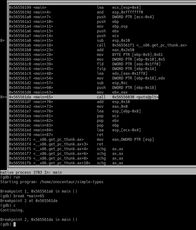 GDB running the simple-types program
We are now going to examine the memory locations where we stored our local variables and try to read the data in them. The first local variable that appears in the code, in line <main+28>, appears to be 1 byte in size. It is referenced as an offset of EBP: ebp-0x9.
==action: Type:==
x $ebp-0x9
Note: The x command defaults to hexadecimal the first time you run it. Thereafter, it defaults to the last data type used. The best approach to avoid confusion is to explicitly tell the command how you would like to read your data.
Tip: Note that you won’t always know what type of data is stored in an address, so be prepared to try a few different formats.
==action: Type:==
x /c $ebp-0x9
We are now telling the x command to read the data as an ASCII character. The output makes more sense:
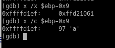 Examining the contents of a memory address containing a single character
Following the example above, let’s check what is stored in our next local variable: ebp-0x10.
==action: Type:==
x /d $ebp-0x10
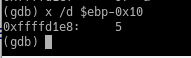 Examining the contents of a memory address containing an unsigned integer
The /d specifier reads the data as an unsigned decimal.
The next local variable, ebp-0x14, is of type float. For the sake of precision, we will specify the size of the data as a word (2 bytes), as well as the format.
==action: Type:==
x /fw $ebp-0x14
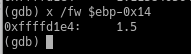 Examining the contents of a memory address containing a floating-point number
Action: Read the data stored in the remaining local variable using an appropriate format specifier.
Hint: you will need to use x to read the data as an address, then use x again to read the data at the address returned as a string. Feel free to consult the GDB Quick Reference.
CTF Challenges
Now that we have had a brief introduction to GDB, let’s jump straight into this week’s CTF challenges. There are 5 challenges this week, designed to teach you different skills in GDB as you progress through them. There is often more than one way in which you can achieve the same results - feel free to explore them.
General tips
Flag: For all the challenges, once you have found the password, run the program again outside of GDB to get your flag.
Tip: If at any point your console layout looks jumbled, with the text you type overwriting the text on the screen, hit Ctrl + L to fix it.
Remember to use:
| run | execute the program from within GDB |
|---|---|
si |
“step into” the next assembly instruction |
ni |
“step over” the next assembly instruction (don’t step into functions) |
fin |
“step out” of the function |
c |
continue, or “play” |
GdbIntro
Hint: This is a nice guided introduction to GDB. Once you have identified the correct call to strcmp(), check the values pushed to the stack just before the function is called.
GdbRegs
Hint: An alternative to the instructions provided is to add a breakpoint at the end of the retval_in_rax() function and use the REGS layout to display the registers. Another option is to use “info registers” or “info registers” + the name of the register you are interested in. Remember that RAX is the 64-bit version of EAX.
GdbSetmem
Hint: Set a breakpoint on the line that does the cmp. When the code stops there, find out what values are being compared. Change one of them using the set command so the jump is not taken and the password is printed on the screen.
GdbPractice
Hint: Put a breakpoint at the start of pwdFunction(). When the execution stops, examine the value in EAX. Remember to read it as a string.
GdbParams
Hint: Once you have identified the function you are interested in, break just before the function is called and examine its arguments (the strings pushed to the stack). The password is one of them.
Conclusion
At this point you have:
- Been introduced to dynamic malware analysis and learned the importance of performing this type of analysis in a secure environment;
- Understood the difference between basic and advanced dynamic analysis;
- Learned how to use GDB to step through a program’s execution at assembly level, without having access to the source code;
- Solved practical CTF challenges and found 5 more flags!
Well done!
GDB is a powerful tool for performing dynamic analysis on malware for which the source code is not available. Now that you have completed this lab’s work, you are ready to take on more advanced debugging challenges.