Ghidra Software Reverse Engineering (SRE)

Introduction

In this lab we dive into the powerful software reverse engineering (SRE) tool, Ghidra. Ghidra was created and is maintained by the National Security Agency Research Directorate. It existed in secret for around 20 years, and in 2019 it was released as free and open source software. Ghidra can perform disassembly, assembly, decompilation, and graphing, and has support for scripting, and runs on Java, compatible with running on Linux, Windows, or Mac OS X, and can analyse a large number of binary architectures.

In this lab we will review the C and assembly language relationship, review how to interpret disassembled and decompiled code, and look at some of the features of Ghidra and its interface.

Hello, world!

Ghidra’s strength is the ability to analyse programs without access to the high level source code (such as C or C++) used to generate the binary machine language.

However, to build our familiarity with Ghidra, it’s useful to generate some our own programs to analyse, so we can compare the original source to assembly and binary process, and how that translates to information that Ghidra presents to you, for you to interpret and use.

==action: Create a hello_world.c file with this content:==

#include <stdio.h>

int main()
{
  printf("Hello, world!\n");
  return 0;
}

Compile a 64 bit executable:

gcc -o hello_world hello_world.c

Compile a 32 bit executable:

gcc -m32 -o hello_world_32 hello_world.c

Compile a 32 bit executable without support for layout randomisation:

gcc -m32 -fno-pie -no-pie -o hello_world_32_no_pie2 hello_world.c

Starting with Ghidra

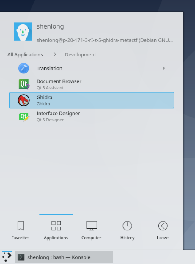
In your VM, Ghidra is pre-installed, it can be found in the Applications Menu under “Development”.

==action: Start Ghidra via the Applications Menu.==

After accepting the terms, the Ghidra Project Window will open.

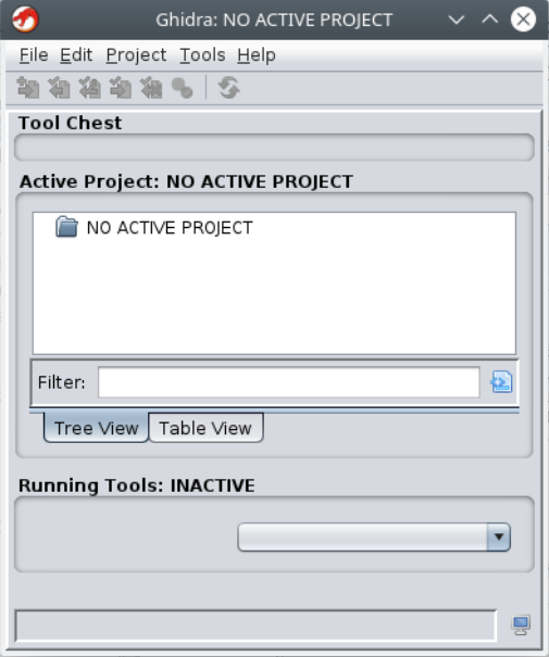
Ghidra is project oriented, so you start a project before you can do analysis.

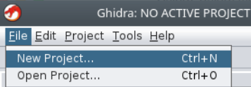
==action: Click the File Menu, to start a “New Project”.==

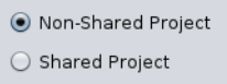
Ghidra has features to collaborate with others on analysis, however, we are not going to explore that feature, so you can select “Non-Shared Project”:

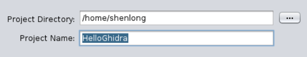
==action: Name your project, for example “HelloGhidra”:==

Your project starts with the CodeBrowser and VersionTracking tools selected:

To start you need to import files into your project.

==action: Click File Menu → Import File (or simply press the “I” key as a shortcut).==

Tip: For a list of shortcuts in Ghidra: https://ghidra-sre.org/CheatSheet.html

==action: Browse to the hello_world executable file you created earlier.==

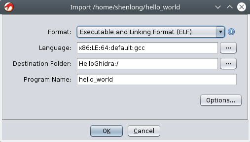
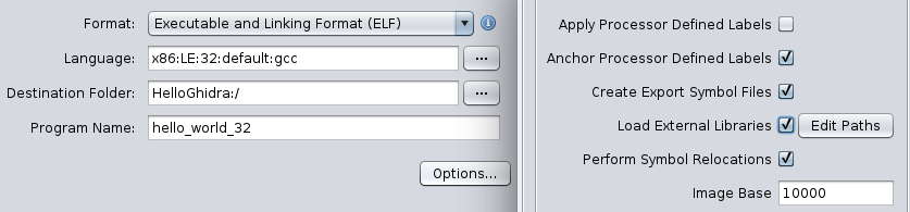
When you add the file, it does a good job of automatically detecting the architecture of the executable – in this case x86 processor, little endian, 64bit. ==action: Click OK to import the file.==

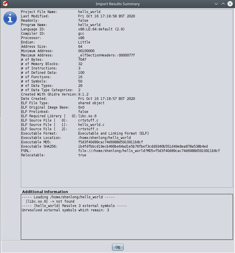
Ghidra will present an overview of the file that has been imported. Take a moment to read through the information that is presented.

Make a note that there is a required library that this program uses: libc.so.6

==action: Double-click on the file to open it.==

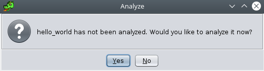
Each time you import a program, Ghidra will prompt you to run analysis on the file. Normally you would do so, but to get a good idea what’s happening,

==action: select “No”:==

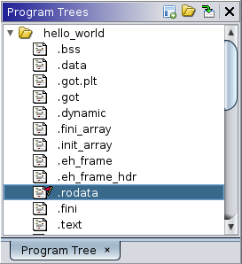
At the top left you will notice a “Program Trees” window, which shows the program sections, ==action: navigate to the .rodata section, by double-clicking:==

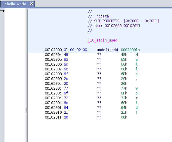
In its un-analysed view it simply lists the individual bytes along with an ASCII representation. Reading down the column you can see our hello world message:

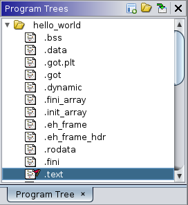
==action: Browse to the .text section (again double clicking the Program Tree):==

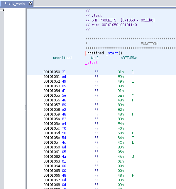
Again, here before analysis we simply have a list of bytes, in hex, along with an ASCII representation, which doesn’t mean much as this is machine code:

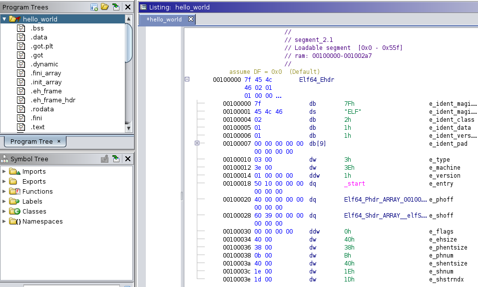
==action: Double-clicking on the root of the tree in the Program Tree shows the whole executable file.==

==action: Read the start of the file. Is this what you expect of an ELF file?==

You should see the ELF magic number 7F 45 4C 46 at the very beginning, which corresponds to the bytes 0x7F, "ELF". This confirms that you’re looking at a valid ELF executable.

You can scroll down through the file, and notice that each section is denoted with a block comment. These sections correspond directly to the ELF sections:

• The .text section contains your program’s machine code
• The .rodata section contains read-only data like string literals
• The .data section contains initialized global variables
• The .bss section contains uninitialized global variables

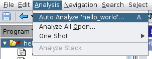
==action: Time to let Ghidra shine. Run the analysis via the “Analysis” menu → “Auto Analyse ‘hello_world’.”==

You will be prompted to select which analyzers to use.

Note: Generally it’s a good idea to include all or most of the stable (non-red) analyzers. The default list may exclude some stable analyzers that take longer to complete. You have the option to re-run analysis, to add additional ones afterwards.

==action: Click “Analyze”.==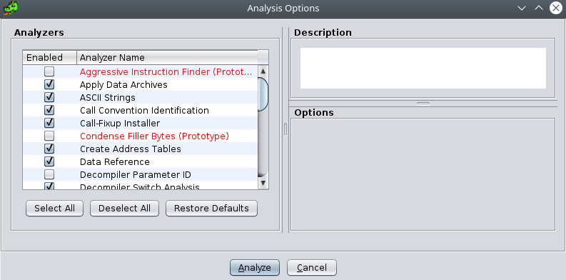

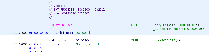
==action: Now, browse back to the .rodata section.== Note that the layout has been updated to include multiple bytes in a single statement, now displaying the string “Hello, world!”.

Note that it has named the constant “s_Hello_world!_” followed by the address of the definition (left-most value, here “00102004”).

This is a perfect example of how Ghidra interprets ELF sections. The .rodata section contains read-only data (like our string literal), and Ghidra has automatically:

1. Detected the data type: Recognized this as a string
2. Named the constant: Created a meaningful symbol name
3. Showed the address: Displayed where this data is located in memory
4. Provided context: Included the actual string content as a comment

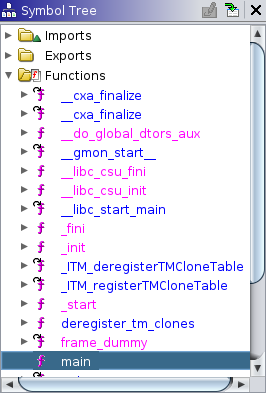
The “Symbol Tree” (middle left) window has a list of functions that have been detected in the program. The pink functions are potential entry points to the program. Later we will return to making sense of the various functions listed. ==action: View the main function (by double clicking it):==

The main function has been disassembled:

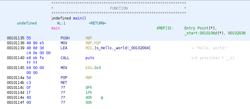
The function starts with a standard function prologue (creating a new stack frame for the function). In this case 64bit code:

PUSH RBP ; this pushes the current base pointer onto the stack, so it can be restored later

MOV RBP, RSP ; sets the base pointer to the value of the stack pointer (top of the stack, so our new stack frame will sit on top of the stack)

Next a value is put into a register to pass a parameter to the function we are about to call. On x86-64 the default register for this happens to be RDI. The actual value placed there is the address of our hello world string. Note that Ghidra uses the automatically generated name s_Hello_world!_address, and also includes the string value as an end of line comment.

LEA RDI,[s_Hello,_world!_00102004] ; copies the address of the hello world constant to the RDI register

Then we call the puts function:

CALL puts ; runs the function, which knows to find the function parameter in RDI

Next the return value (0) is copied to the EAX function, the stack base pointer is restored, and we return from this function:

MOV EAX,0x0 ; return value stored

POP RBP ; restore stack pointer

RET ; return from function

Not only does Ghidra provide disassembly, but it also provides a powerful decompiler -- perhaps one of its most stand-out features.

To the right of the assembly “Listing” window, is the “Decompile” window. ==action: View the decompiled C code:==

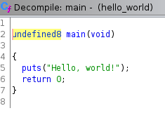
This provides a readable interpretation of the assembly code (which was based on the compiled machine code).

It’s worth noting that the code has ended up similar, but different to the original C code.

The return data types are not correct, and the decompiled program calls the puts function, rather than printf.

Question: What is the difference between the puts function and the printf function? Why does the assembly code call the puts function rather than printf? (Hint GCC performs optimisations.)

Connecting ELF Structure to Assembly Analysis

Now that you understand both ELF structure and assembly code, let’s connect the dots:

==action: In the assembly listing, look at the instruction that loads the string address:==

LEA RDI,[s_Hello,_world!_00102004]

This instruction is loading the address of our string from the .rodata section. The address 00102004 corresponds to where Ghidra found our “Hello, world!” string in the ELF file.

==action: Compare this with what you saw in the .rodata section earlier. The address should match the location where Ghidra displayed the string.==

This demonstrates how:

1. ELF sections organize different types of data in the file
2. Assembly instructions reference data by memory addresses
3. Ghidra bridges the gap by showing both the raw bytes and their interpreted meaning

Question: Can you identify which ELF section contains the machine code for the main function? (Hint: Look at the Program Trees window and find where the assembly instructions are located.)

32 and 64 bit CPU architectures, and memory layout randomisation

It’s helpful at this point to understand and appreciate that the compiler is making various decisions about the actual details of the assembly code, and the assembly code generated will differ based on various compiler options, and the target architecture (CPU instructions and registers are architecture dependant, for example, x86 has a different set of instructions compared to ARM CPUs), and operating system, as different standard libraries will be used and available.

There are many valid ways the compiler could decide to generate the program, and the output will reflect a number of decisions made by the compiler. For example, view this list of gcc optimisation options: https://gcc.gnu.org/onlinedocs/gcc/Optimize-Options.html

Earlier you also compiled a 32-bit version of the hello world program.

==action: Import the hello_world_32 program into the project (you can use the “I” keyboard shortcut, or use the menu).==

==action: This time when you are importing it, click Options, and select “Load External Libraries”.==

==action: Run the default analysis.==

==action: Browse to the main function.==

Note that the compiled program’s assembly is a fair bit more complicated than the 64bit version -- this is because the compiler is adding support for features that are already there as part of the 64bit architecture.

The main function often needs to do additional setup and cleanup that other functions do not need to, including reading command line arguments into the program. Some of the additional code is sometimes related to stack alignment (an optimisation around the starting position for where on the stack the values are placed), and to support position-independent executables (PIE).

Most notably if you view the decompiled view, depending on the compiler, there may be an extra function being called, __x86.get_pc_thunk.ax:

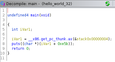
The __x86.get_pc_thunk.ax function is used to accommodate PIE, which means the program machine code can be loaded at any address in virtual memory and it will still be able to run.

PIE means the program can support address space layout randomization (ASLR), which randomises the layout for increased security, as it makes exploitation of memory vulnerabilities more difficult.

==action: Import the hello_world_32_no_pie program, run the default analysis, and browse to the main function.==

Question: How do these three versions of the same program differ?

==tip: Note that a lot of this additional code only gets added once to the main function, so it helps to be familiar with it, so you can concentrate on the rest of the program.==

Program startup and boiler plate code

As you browse through the code, you may have noticed that there are a lot of functions that seem unrelated to our main function: scroll down the Symbol Tree for some examples. These are used to perform program startup and teardown. On a Linux ELF, the entry point is defined in a header, which normally points to the _start function, which in turn calls a number of functions to set up the program, and then finally runs the main function, where the program specific code is located.

==tip: For the challenges in this module we will typically stick to this convention/standard, so it is safe to ignore these for the most part – however, you should be aware that malware does not always stick to conventions.== Also this list of supporting functions is specific to Linux, and Windows or Mac executables have their own standard set of functions.

Here is a handy diagram of some of the functions that are typically used to start a ELF program:

This diagram, and a detailed description of the startup process can be found here:

https://web.archive.org/web/20191210114310/http://dbp-consulting.com/tutorials/debugging/linuxProgramStartup.html

https://stackoverflow.com/questions/34966097/what-functions-does-gcc-add-to-the-linux-elf/34973886

Thunk functions and external libraries

==action: In the 64bit hello_world, double click on the puts function.==

Note that this takes you to a “thunk function”, which is essentially a function stub that gets linked to an external library call:

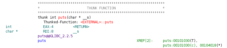
In this case, we didn’t choose the option when importing, to load the external library, so we can’t easily access the puts function to see what it’s doing.

If you followed the instructions above carefully, you will have chosen to import the external libraries when loading the 32bit version, so ==action: in hello_world_32, double click on the puts function:==

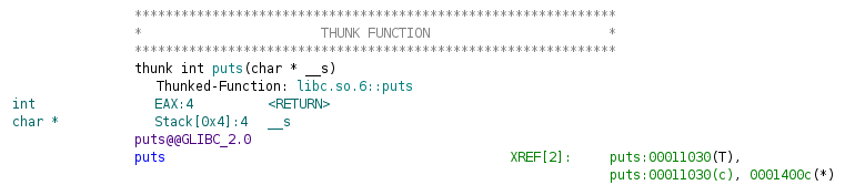
Now, since you linked the shared library, you can follow the reference to load the library for analysis. ==action: Double click on the teal-coloured “libc.so.6::puts”.==

You don’t need to run analysis on this file, unless you want to.

Lab CTF challenge 1

We return to the “Ch1_Readelf” challenge.

==action: Import the challenge (including external libraries), and navigate to the main function.==

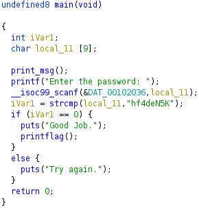
You should see the power of the decompiler in full force here, the generated code is pretty clear, including the solution to the challenge.

==action: Run the challenge binary and enter the password to get your flag.==

Detailed analysis via annotating and commenting code

While the decompiler output for the above Ch1_Readelf challenge is good, it could be clearer, and when the amount of code involves a large number of local randomly named variables (often not detected as the correct data type) it can be much harder to read without recording the progress of your analysis.

We will now go through the process of analysing this binary in more detail, to produce a more human readable output, including variable names and comments.

An effective approach to analysis is to work on creating self-documenting reverse engineered code -- the end result is reverse engineered code that is well documented and easier to read and understand (while still accurately representing the underlying machine code and assembly instructions).

The difficulty and amount of work will depend on whether the program is externally linked, whether symbols have been included, and whether the code has been intentionally obfuscated.

In this case, the function names print_msg, and printflag give clear clues to the purpose of these. In this case, the binary symbol table hasn’t been stripped.

As a general approach it is helpful to iteratively improve the readability of the code by:

• Rename functions and signatures
• Work back from library calls (look at external documentation) to name parameters and return variables
• Rename variables
• Add comments

Rename functions and function signatures, and renaming variables

Note that the main function hasn’t been detected correctly.

Almost always the first thing to do is redefine the main function and its parameters. For C code on Linux, it should always read:

int main(int argc, char **argv)

Tip: Alternatively written as int main(int argc, char *argv[]), however, Ghidra insists on the char** notation for a pointer to an array.

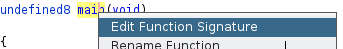
==action: Update the function signature, by right clicking main function name, then click “Edit Function Signature”:==

Note that now the assembly for reading the command line arguments is clearer (although in this program the arguments are not actually used later).

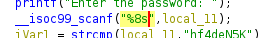
Next, as we read down the code, the function, __isoc99_scanf could be renamed to scanf to improve readability (isoc99 is a specific C specification version). Also looking at the parameters, we can see that the datatype of the first parameter (here DAT_00102036) has not been detected.

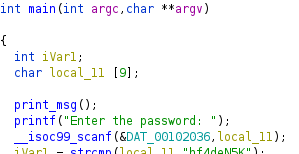
==action: Double click on the first parameter (DAT_00102036).== This will navigate you to the .rodata section, where this constant is defined:

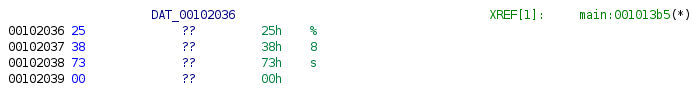
Clearly this parameter represents the format string “%8s”, yet Ghidra doesn’t know what to make of this.

There are a few different approaches we can take to remedy this. One approach is to set its type here in .rodata.

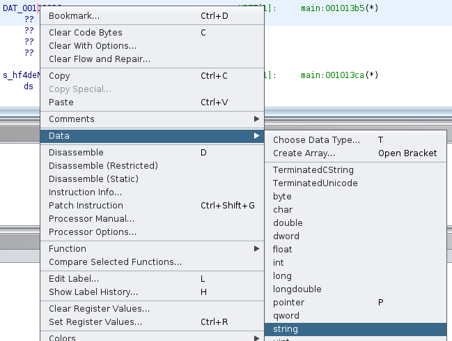
==action: Right click the constant name (DAT_00102036) and click “Data” → “string”.== (Or use the shortcut “T”)

This will automatically relabel the variable, and in the decompiler you will see the function call has become more readable by showing the constant string in place:

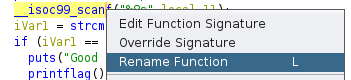
==action: We can rename the function “scanf”, by right clicking the name, and click “Rename Function”== (or shortcut “L”)

Note: You can press Ctrl-Z twice to undo your last two changes.

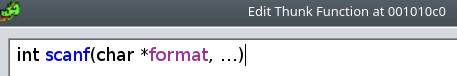
We can Edit Function Signature for scanf. A quick Google will give you the actual signature for this function:

int scanf(const char *format, ...)

https://www.man7.org/linux/man-pages/man3/scanf.3.html

Or at the command line “man scanf”

Ghidra doesn’t accept the above without removing the “const”:

==action: Save the new function signature.==

This renames the function AND also sets the datatype. (We needn’t have done the previous two steps.)

Scanf is a variadic function: the “…” represents that the function can be sent any number of additional parameters. Reading the documentation for scanf explains that the format string tells it how many parameters to expect. In this case the format string “%8s” means that it should read one string up to 8 characters long, and store it in the following char* variable.

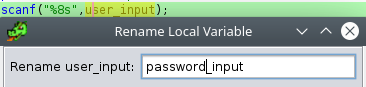
Based on this information (and looking at the context of the call in the main function) we can rename the second parameter (local_11).

==action: Right click on the second parameter to scanf in the main function, and click “Rename Local Variable”== (or shortcut “L”), and enter “password_input”:

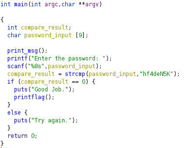
The strcmp return value can be renamed to “compare_result”, and we are left with a main function that is clear and easy to follow:

Comments

While the above is clear, and arguably already very readable, it’s often helpful to add comments during your analysis, especially to add clarity to complex logic, explaining the behaviour you have identified.

There are a few different types of comments that get displayed in various places, including the Listing and Decompile views.

Let’s explore what each type of comment is.

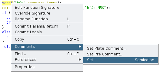
==action: Right click on the scanf line, and select “Comments” → “Set…”:==

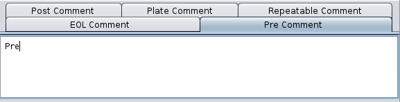
==action: Click on each tab and enter in the first word from the title of the tab, as the comment to add:==

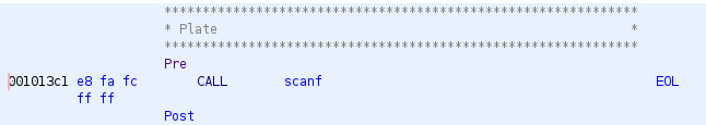
The listing view has been updated showing plate, pre, post, and EOL comments:

The decompiler view only shows the pre comment:

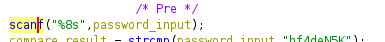
==action: View the .ro_data section, and find where the password is defined (or double click it in main), and set a repeatable comment: “the solution!”.== View the assembly for main, and find the comment repeat where the constant is used.

Flag: Run the challenge executable with the password for the flag!

Lab CTF challenge 2

Flag: Use what you have learned to solve the second flag.

Hint: The second challenge may take a while to figure out. Use everything you have learned above to make the process easier, by renaming variables and adding comments for clarity. It is standard practice to use short one letter variable names for simple iteration counters, for example, i, for the first loop, then inner loops named j, k, l, and so on.

Tip: Be sure to include the results of your Ghidra analysis for this challenge in your log book, including the decompiled source code with renamed variables and comments.

Conclusion

At this point you have:

• Used Ghidra, a powerful reverse software engineering tool
• Become familiar with some of Ghidra’s most common features, including navigating program sections using the Program Trees window, the Symbol Tree to browse to functions, the Listing view for disassembly code, and the Decompile window.
• Explored (and started to build some familiarity) with the ELF files and assembly for 64 and 32 bit Linux executables, and the various boilerplate code, and the purpose of thunk functions.
• Learned how to start performing advanced analysis, by working through decompiled and disassembled code, defining function signatures, renaming variables, setting simple data types, and adding different types of comments to aid clarity.
• Solved practical CTF challenges and found 2 more flags!

Well done!